Amdahl’s Law vs. Gustafson’s Law — Full Tutorial with Derivations, Use Cases, and Python Plot

Amdahl’s Law vs Gustafson’s Law: Full Tutorial, Derivations, Use Cases, and Python Plot
Understanding Parallel Speedup: Amdahl’s Law and Gustafson’s Law Explained with Code
Parallel Computing Essentials: Amdahl’s Law, Gustafson’s Law, and Speedup Modeling
How Parallel Speedup Works: Complete Guide to Amdahl’s and Gustafson’s Laws
Parallel Scaling Explained: Deriving and Comparing Amdahl’s and Gustafson’s Laws
Amdahl vs Gustafson: The Complete Guide to Parallel Speedup (with Python Code)
Parallel Performance Modeling: Amdahl’s Law, Gustafson’s Law, and Real-World Use Cases
Learn Parallel Speedup: Math, Intuition, Use Cases, and Python Visualization
Parallel Computing: The Two Laws You Must Know (Amdahl & Gustafson)
Parallel Speedup for Engineers: Amdahl’s Law, Gustafson’s Law, and Python Implementation
From Theory to Code: Modeling Parallel Speedup with Amdahl and Gustafson
A Practical Guide to Parallel Speedup: Amdahl’s Law, Gustafson’s Law, and Visualization
Why Parallelism Isn’t Infinite: Amdahl vs Gustafson Explained Simply
The Truth About Parallel Speedup: Amdahl’s Limits vs Gustafson’s Scaling
Parallel Computing Myths vs Reality: What Amdahl and Gustafson Teach Us

Introduction

Parallel computing is essential in modern computing: multi-core CPUs, GPUs, distributed clusters, cloud workloads, LLM training, and HPC simulations.
To reason about how much faster a program becomes with more processors, two mathematical models dominate:

• Amdahl’s Law — fixed-size workload performance
• Gustafson’s Law — scaled-size workload performance

These two laws are not contradictory. They answer different questions.
This tutorial covers derivations, intuition, comparisons, practical use cases, and a Python plotting script showing both laws together.

1. What Is Speedup?

Speedup measures how much faster a program runs with N processors:

If a program takes 10 seconds on one processor and 5 seconds on two, speedup is:

Perfect linear speedup would be:

But real systems contain serial bottlenecks. This is what Amdahl’s and Gustafson’s laws describe.

2. Amdahl’s Law (Fixed Workload)

2.1 Intuition

Amdahl assumes:

• The total amount of work stays the same
• A portion is serial and cannot be parallelized

Let:

• f = serial fraction
• 1 - f = parallel fraction

2.2 Derivation

Time on one processor:

Define:

Thus:

Time on N processors:

Speedup:

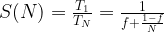
Where f is the portion of the serial work and is the work that can be parallelized. Amdahl’s formula can be also rewritten as using :

As and

2.3 Limit as N → ∞

If the serial fraction is 10% (f = 0.1):

Even infinite processors cannot exceed that.

2.4 Practical Use Cases for Amdahl’s Law

Amdahl is ideal when optimizing latency for a fixed task:

• GPU kernel optimization for fixed tensor size
• Reducing inference latency for a single request
• Video encoding, compression, sorting
• Making a fixed-size batch job run faster
• Database query acceleration

---

3. Gustafson’s Law (Scaled Workload)

3.1 Intuition

Gustafson reverses the question:

“With more processors, how much larger a problem can I solve in the same time?”

This reflects real HPC workloads: more CPUs → finer resolution → bigger simulations.

3.2 Derivation

Assume the program runs in 1 time unit on N processors.

Let:

• f = serial fraction (measured at scale)

The parallel portion scales with the number of processors, so its runtime remains proportional to N.

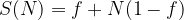
Time on one processor:

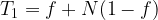
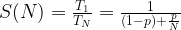
Thus, the speedup is:

We can re-write Gustafson’s formula in “N minus” form:

Or, if we define the parallel fraction as , the formula can also be written as:

Now the “N minus” form in terms of p becomes:

3.3 Interpretation

As N increases, speedup approaches:

This is nearly linear for small serial fractions.

3.4 Practical Use Cases for Gustafson’s Law

Use Gustafson for throughput scaling or workloads where you can increase problem size:

• Weather and climate simulations
• Particle simulations, CFD, finite element analysis
• LLM training: more GPUs → longer sequences or bigger models
• Big data analytics (Spark, Dask, Flink)
• Monte Carlo simulations

---

4. Amdahl’s Law vs. Gustafson’s Law (Comparison Table)

Item	Amdahl	Gustafson
Workload	Fixed	Scales with N
Goal	Reduce latency	Increase throughput
Speedup limit	Bounded:	Nearly linear:
Pessimistic/Optimistic	Pessimistic	Optimistic
Use cases	Optimizing existing tasks	Scaling larger workloads

---

5. Practical Use Cases (Combined View)

Amdahl (Latency Optimization)

• Reducing inference time for one LLM query
• Speeding up database joins
• GPU kernel tweaks for fixed tensors
• Video encoding (same video)

Gustafson (Throughput / Scale)

• LLM training (scale to more GPUs)
• Simulating higher-resolution weather models
• Big data ETL scaling
• Scientific HPC workloads

6. Python Script to Plot Both Laws

The code below generates a graph showing Amdahl’s and Gustafson’s speedup curves.

You can adjust f (serial fraction) and the number of processors N.

The following script plots Amdahl and Gustafson speedup curves on the same graph.

It includes a few values of e.g. the serial portion:

import numpy as np
import matplotlib.pyplot as plt

def amdahl_speedup(N, s):
    return 1.0 / (s + (1 - s) / N)

def gustafson_speedup(N, s):
    return s + (1 - s) * N

# Number of processors
N = np.arange(1, 65)

# Serial fractions to consider
Serial = [0.05, 0.1, 0.2, 0.3, 0.5, 0.8, 0.9, 1.0]

plt.figure(figsize=(10, 6))

for f in Serial:
    plt.plot(N, amdahl_speedup(N, f), linestyle='-', label=f"Amdahl Serial={f}")
    plt.plot(N, gustafson_speedup(N, f), linestyle='--', label=f"Gustafson Serial={f}")

plt.title("Amdahl's Law")
plt.xlabel("Number of Processors (N)")
plt.ylabel("Speedup")
plt.legend()
plt.grid(True)
plt.tight_layout()

plt.savefig("parallel-speedup-amdahl-vs-gustafson.png")
## plt.show()

Here are the plots of the Amdahl’s vs Gustafson.

Interpreting the Plots

• Amdahl curves flatten quickly—bottlenecked by the sequential portion.
• Gustafson curves rise almost linearly—useful when workloads can scale.
• Higher f increases the gap between the two models.

Conclusion

Amdahl’s Law shows the limits of parallelism for fixed workloads, making it ideal for latency optimization. Gustafson’s Law shows the opportunities of parallelism when workloads scale with compute.

• Amdahl’s Law → fixed-size workloads → diminishing returns
• Gustafson’s Law → scalable workloads → near-linear speedup
• Use both to understand hardware limits and the nature of your algorithm
• Python tools make visualization simple and intuitive

Together, they form the foundation of reasoning about performance in modern parallel systems, from HPC to LLM training to GPU compute.

–EOF (The Ultimate Computing & Technology Blog) —

2531 words
Last Post: Teaching Kids Programming - Introduction to Combinatorial Mathematics 1 (Pascal Triangle/Binomial)
Next Post: Understanding the Sigma Function: Divisors, Multiplicativity, and the Formula