This article explains how to approximate Pi using the definite integral
. It introduces the mathematics behind the identity, explains the trapezoidal and midpoint integration methods, and provides single-threaded and multithreaded implementations in both Python and C++. It also demonstrates how the same calculation can be divided across five distributed computing nodes, with a discussion of numerical accuracy, performance, parallelism, and practical limitations.
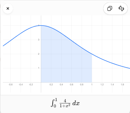
The Definite Integral Computes the Pi
Pi, written as  , appears throughout mathematics, physics, engineering, statistics, and computer science. Although programming languages normally provide a built-in value of Pi, calculating it ourselves is a useful way to learn about calculus, numerical integration, multithreading, and distributed computing.
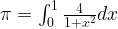
In this article, we will calculate Pi using the definite integral:
We will cover:
- Why the integral equals Pi
- How numerical integration approximates an integral
- The trapezoidal rule
- The midpoint rule
- Single-threaded Python
- Multithreaded Python
- Single-threaded C++
- Multithreaded C++
- How the same algorithm can be distributed across five nodes
Why Does This Integral Equal Pi?
Consider the integral:

The key observation is that the derivative of the inverse tangent function is:

Therefore:

Applying the limits from zero to one gives:

This means:

We know that:

and:

Therefore:

So:
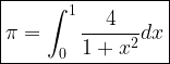
This gives us a convenient way to calculate Pi numerically.
How Numerical Integration Works
A computer does not need to solve the integral symbolically. Instead, it can divide the interval into many small pieces and approximate the area under the curve.
Suppose we want to calculate:
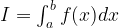
Divide the interval  into
into  equal subintervals.
The width of each interval is:

The points dividing the interval are:

where:

There are several ways to approximate the area of each small section. Two common methods are:
- The trapezoidal rule
- The midpoint rule
The Trapezoidal Rule
The formula involving  ,
,  , and division by two is the trapezoidal rule.
For one interval from  to
to  , the function is approximated by a straight line. The resulting shape is a trapezoid.
Its area is:

Adding the areas of all trapezoids gives:

An equivalent and often easier-to-implement form is:
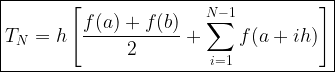
The two endpoints receive half weight:

All interior points receive full weight:

For our Pi integral:

and:

Therefore:

The trapezoidal approximation becomes:

Since:

and:

we can also write:

A Small Trapezoidal Example
Suppose we use four intervals:

The interval width is:
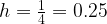
The five boundary points are:

The function values are approximately:





Applying the trapezoidal formula:

Therefore:

The actual value is:

Using only four intervals already gives a reasonable approximation. Increasing improves the result.
The Midpoint Rule
The implementations later in this article primarily use the midpoint rule.
Instead of evaluating the function at the boundaries of each interval, the midpoint rule evaluates it at the centre.
The midpoint of interval  is:
is:

The area of that interval is approximated by a rectangle:

Adding all rectangles gives:
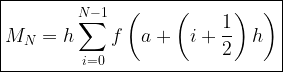
For the Pi integral,  ,
,  , and
, and  .
.
Therefore:
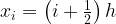
and:
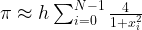
Substituting :
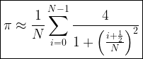
The larger becomes, the closer the estimate gets to Pi.
Trapezoidal Rule Versus Midpoint Rule
| Method | Sample positions | Formula |
|---|---|---|
| Trapezoidal rule | Interval boundaries |  |
| Midpoint rule | Centre of each interval |  |
For a smooth function, both methods normally have an error proportional to:

However, the midpoint rule is often more accurate than the trapezoidal rule when both use the same number of intervals.
Single-Threaded Python Using the Midpoint Rule
The following Python program uses 25 million intervals.
import math
import time


def calculate_pi(total_steps: int) -> float:
    if total_steps <= 0:
        raise ValueError("total_steps must be positive")

    step_width = 1.0 / total_steps
    total = 0.0

    for step in range(total_steps):
        midpoint = (step + 0.5) * step_width
        total += 4.0 / (1.0 + midpoint * midpoint)

    return total * step_width


def main() -> None:
    total_steps = 25_000_000

    started_at = time.perf_counter()
    pi_estimate = calculate_pi(total_steps)
    elapsed_seconds = time.perf_counter() - started_at

    absolute_error = abs(pi_estimate - math.pi)

    print(f"Estimated Pi:   {pi_estimate:.15f}")
    print(f"Reference Pi:   {math.pi:.15f}")
    print(f"Absolute error: {absolute_error:.3e}")
    print(f"Elapsed time:   {elapsed_seconds:.3f} seconds")


if __name__ == "__main__":
    main()
The core calculation is:
midpoint = (step + 0.5) * step_width
total += 4.0 / (1.0 + midpoint * midpoint)
The first line calculates the midpoint of the current interval:
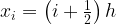
The second line evaluates:
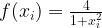
After all values have been added, the result is multiplied by the interval width:
return total * step_width
Mathematically, this calculates:
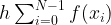
Single-Threaded Python Using the Trapezoidal Rule
The trapezoidal version evaluates the function at the interval boundaries rather than at the midpoints.
import math
import time


def calculate_pi_trapezoidal(total_steps: int) -> float:
    if total_steps <= 0:
        raise ValueError("total_steps must be positive")

    h = 1.0 / total_steps

    def f(x: float) -> float:
        return 4.0 / (1.0 + x * x)

    total = 0.5 * (f(0.0) + f(1.0))

    for step in range(1, total_steps):
        x = step * h
        total += f(x)

    return total * h


def main() -> None:
    total_steps = 25_000_000

    started_at = time.perf_counter()
    pi_estimate = calculate_pi_trapezoidal(total_steps)
    elapsed_seconds = time.perf_counter() - started_at

    absolute_error = abs(pi_estimate - math.pi)

    print(f"Estimated Pi:   {pi_estimate:.15f}")
    print(f"Reference Pi:   {math.pi:.15f}")
    print(f"Absolute error: {absolute_error:.3e}")
    print(f"Elapsed time:   {elapsed_seconds:.3f} seconds")


if __name__ == "__main__":
    main()
The endpoint contribution is calculated by:
total = 0.5 * (f(0.0) + f(1.0))
This corresponds to:

The loop calculates the interior sum:
for step in range(1, total_steps):
    x = step * h
    total += f(x)
This corresponds to:

Finally, the total is multiplied by  :
:
return total * h
Multithreaded Python Using the Midpoint Rule
We can divide the 25 million intervals among five workers.
For worker  out of
  workers, the start index is:
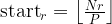
The end index is:
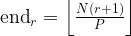
For five workers and 25 million intervals:
| Worker | Start step | End step | Number of steps |
|---|---|---|---|
| 0 | 0 | 5,000,000 | 5,000,000 |
| 1 | 5,000,000 | 10,000,000 | 5,000,000 |
| 2 | 10,000,000 | 15,000,000 | 5,000,000 |
| 3 | 15,000,000 | 20,000,000 | 5,000,000 |
| 4 | 20,000,000 | 25,000,000 | 5,000,000 |
Here is an implementation using ThreadPoolExecutor:
import math
import time
from concurrent.futures import ThreadPoolExecutor


def calculate_partial_sum(
    start_step: int,
    end_step: int,
    step_width: float,
) -> float:
    partial_sum = 0.0

    for step in range(start_step, end_step):
        midpoint = (step + 0.5) * step_width
        partial_sum += 4.0 / (1.0 + midpoint * midpoint)

    return partial_sum


def calculate_pi_multithreaded(
    total_steps: int,
    worker_count: int,
) -> float:
    if total_steps <= 0:
        raise ValueError("total_steps must be positive")

    if worker_count <= 0:
        raise ValueError("worker_count must be positive")

    step_width = 1.0 / total_steps
    ranges = []

    for worker_id in range(worker_count):
        start_step = total_steps * worker_id // worker_count
        end_step = total_steps * (worker_id + 1) // worker_count
        ranges.append((start_step, end_step))

    with ThreadPoolExecutor(max_workers=worker_count) as executor:
        futures = [
            executor.submit(
                calculate_partial_sum,
                start_step,
                end_step,
                step_width,
            )
            for start_step, end_step in ranges
        ]

        partial_sums = [
            future.result()
            for future in futures
        ]

    return sum(partial_sums) * step_width


def main() -> None:
    total_steps = 25_000_000
    worker_count = 5

    started_at = time.perf_counter()

    pi_estimate = calculate_pi_multithreaded(
        total_steps,
        worker_count,
    )

    elapsed_seconds = time.perf_counter() - started_at
    absolute_error = abs(pi_estimate - math.pi)

    print(f"Workers:        {worker_count}")
    print(f"Estimated Pi:   {pi_estimate:.15f}")
    print(f"Reference Pi:   {math.pi:.15f}")
    print(f"Absolute error: {absolute_error:.3e}")
    print(f"Elapsed time:   {elapsed_seconds:.3f} seconds")


if __name__ == "__main__":
    main()
Each worker calculates one partial sum:

The main thread combines the results:

An Important Python Limitation
The multithreaded Python version demonstrates how to divide the calculation into separate ranges, but it may not execute faster than the single-threaded version.
Standard CPython has a Global Interpreter Lock, commonly called the GIL. For CPU-bound Python code, only one thread normally executes Python bytecode at a time.
Therefore, five Python threads do not necessarily use five CPU cores effectively.
The threaded version may be:
- Approximately as fast as the single-threaded version
- Slightly slower because of thread-management overhead
- Useful for demonstrating work partitioning
- Unsuitable for achieving true CPU parallelism in normal CPython
For true CPU parallelism in Python, better choices include:
ProcessPoolExecutor- The
multiprocessingmodule - NumPy
- Native extensions
- MPI
- Separate distributed processes
Single-Threaded C++ Using the Midpoint Rule
C++ is well suited to tight numerical loops because it compiles directly to native machine code.
#include <chrono>
#include <cmath>
#include <cstdint>
#include <iomanip>
#include <iostream>
#include <stdexcept>


double calculate_pi(std::uint64_t total_steps) {
    if (total_steps == 0) {
        throw std::invalid_argument(
            "total_steps must be positive"
        );
    }

    const double step_width =
        1.0 / static_cast<double>(total_steps);

    double total = 0.0;

    for (
        std::uint64_t step = 0;
        step < total_steps;
        ++step
    ) {
        const double midpoint =
            (static_cast<double>(step) + 0.5)
            * step_width;

        total += 4.0 / (1.0 + midpoint * midpoint);
    }

    return total * step_width;
}


int main() {
    constexpr std::uint64_t total_steps = 25'000'000;

    const auto started_at =
        std::chrono::steady_clock::now();

    const double pi_estimate =
        calculate_pi(total_steps);

    const auto finished_at =
        std::chrono::steady_clock::now();

    const double elapsed_seconds =
        std::chrono::duration<double>(
            finished_at - started_at
        ).count();

    const double reference_pi = std::acos(-1.0);

    const double absolute_error =
        std::abs(pi_estimate - reference_pi);

    std::cout
        << std::fixed
        << std::setprecision(15);

    std::cout
        << "Estimated Pi:   "
        << pi_estimate
        << '\n';

    std::cout
        << "Reference Pi:   "
        << reference_pi
        << '\n';

    std::cout
        << std::scientific
        << std::setprecision(3);

    std::cout
        << "Absolute error: "
        << absolute_error
        << '\n';

    std::cout
        << std::fixed
        << std::setprecision(3);

    std::cout
        << "Elapsed time:   "
        << elapsed_seconds
        << " seconds\n";

    return 0;
}
Compile it with optimisation enabled:
g++ -O3 -std=c++17 pi_single.cpp -o pi_single
Run it using:
./pi_single
The -O3 option enables aggressive compiler optimisation. Without optimisation, the program may run considerably more slowly.
Single-Threaded C++ Using the Trapezoidal Rule
The following C++ version implements the trapezoidal formula:

#include <chrono>
#include <cmath>
#include <cstdint>
#include <iomanip>
#include <iostream>
#include <stdexcept>


double f(double x) {
    return 4.0 / (1.0 + x * x);
}


double calculate_pi_trapezoidal(
    std::uint64_t total_steps
) {
    if (total_steps == 0) {
        throw std::invalid_argument(
            "total_steps must be positive"
        );
    }

    const double h =
        1.0 / static_cast<double>(total_steps);

    double total =
        0.5 * (f(0.0) + f(1.0));

    for (
        std::uint64_t step = 1;
        step < total_steps;
        ++step
    ) {
        const double x =
            static_cast<double>(step) * h;

        total += f(x);
    }

    return total * h;
}


int main() {
    constexpr std::uint64_t total_steps = 25'000'000;

    const auto started_at =
        std::chrono::steady_clock::now();

    const double pi_estimate =
        calculate_pi_trapezoidal(total_steps);

    const auto finished_at =
        std::chrono::steady_clock::now();

    const double elapsed_seconds =
        std::chrono::duration<double>(
            finished_at - started_at
        ).count();

    const double reference_pi = std::acos(-1.0);

    const double absolute_error =
        std::abs(pi_estimate - reference_pi);

    std::cout
        << std::fixed
        << std::setprecision(15);

    std::cout
        << "Estimated Pi:   "
        << pi_estimate
        << '\n';

    std::cout
        << "Reference Pi:   "
        << reference_pi
        << '\n';

    std::cout
        << std::scientific
        << std::setprecision(3);

    std::cout
        << "Absolute error: "
        << absolute_error
        << '\n';

    std::cout
        << std::fixed
        << std::setprecision(3);

    std::cout
        << "Elapsed time:   "
        << elapsed_seconds
        << " seconds\n";

    return 0;
}
Compile it using:
g++ -O3 -std=c++17 pi_trapezoidal.cpp -o pi_trapezoidal
Multithreaded C++ Using the Midpoint Rule
Unlike ordinary CPython threads, C++ threads can execute CPU-bound work simultaneously on multiple processor cores.
The following implementation divides the calculation among five threads.
#include <chrono>
#include <cmath>
#include <cstdint>
#include <iomanip>
#include <iostream>
#include <numeric>
#include <stdexcept>
#include <thread>
#include <vector>


double calculate_partial_sum(
    std::uint64_t start_step,
    std::uint64_t end_step,
    double step_width
) {
    double partial_sum = 0.0;

    for (
        std::uint64_t step = start_step;
        step < end_step;
        ++step
    ) {
        const double midpoint =
            (static_cast<double>(step) + 0.5)
            * step_width;

        partial_sum +=
            4.0 / (1.0 + midpoint * midpoint);
    }

    return partial_sum;
}


double calculate_pi_multithreaded(
    std::uint64_t total_steps,
    std::size_t worker_count
) {
    if (total_steps == 0) {
        throw std::invalid_argument(
            "total_steps must be positive"
        );
    }

    if (worker_count == 0) {
        throw std::invalid_argument(
            "worker_count must be positive"
        );
    }

    const double step_width =
        1.0 / static_cast<double>(total_steps);

    std::vector<std::thread> workers;

    std::vector<double> partial_sums(
        worker_count,
        0.0
    );

    workers.reserve(worker_count);

    for (
        std::size_t worker_id = 0;
        worker_id < worker_count;
        ++worker_id
    ) {
        const std::uint64_t start_step =
            total_steps
            * worker_id
            / worker_count;

        const std::uint64_t end_step =
            total_steps
            * (worker_id + 1)
            / worker_count;

        workers.emplace_back(
            [
                &,
                worker_id,
                start_step,
                end_step
            ]() {
                partial_sums[worker_id] =
                    calculate_partial_sum(
                        start_step,
                        end_step,
                        step_width
                    );
            }
        );
    }

    for (std::thread& worker : workers) {
        worker.join();
    }

    const double combined_sum =
        std::accumulate(
            partial_sums.begin(),
            partial_sums.end(),
            0.0
        );

    return combined_sum * step_width;
}


int main() {
    constexpr std::uint64_t total_steps = 25'000'000;
    constexpr std::size_t worker_count = 5;

    const auto started_at =
        std::chrono::steady_clock::now();

    const double pi_estimate =
        calculate_pi_multithreaded(
            total_steps,
            worker_count
        );

    const auto finished_at =
        std::chrono::steady_clock::now();

    const double elapsed_seconds =
        std::chrono::duration<double>(
            finished_at - started_at
        ).count();

    const double reference_pi = std::acos(-1.0);

    const double absolute_error =
        std::abs(pi_estimate - reference_pi);

    std::cout
        << "Workers:        "
        << worker_count
        << '\n';

    std::cout
        << std::fixed
        << std::setprecision(15);

    std::cout
        << "Estimated Pi:   "
        << pi_estimate
        << '\n';

    std::cout
        << "Reference Pi:   "
        << reference_pi
        << '\n';

    std::cout
        << std::scientific
        << std::setprecision(3);

    std::cout
        << "Absolute error: "
        << absolute_error
        << '\n';

    std::cout
        << std::fixed
        << std::setprecision(3);

    std::cout
        << "Elapsed time:   "
        << elapsed_seconds
        << " seconds\n";

    return 0;
}
Compile it with thread support and optimisation:
g++ -O3 -std=c++17 -pthread pi_multithreaded.cpp -o pi_multithreaded
Then run it:
./pi_multithreaded
Why Each Thread Uses a Local Sum
Inside each thread, the program calculates into a local variable:
double partial_sum = 0.0;
It does not update one shared global total during every iteration.
If every thread repeatedly updated the same variable, the program would need a mutex or atomic operation. That would introduce synchronisation and contention.
Instead, the program follows a map-and-reduce pattern:
- Assign one range of intervals to each worker.
- Let each worker calculate independently.
- Store one partial result per worker.
- Wait for all threads to complete.
- Add the partial results together.
Mathematically:

The final approximation is:

Extending the Algorithm to Five Distributed Nodes
Multithreading and distributed computing use the same mathematical partitioning, but they are different execution models.
Threads normally:
- Run on one machine
- Share the same memory
- Belong to the same process
- Communicate through shared variables
Distributed workers normally:
- Run as separate processes
- May run on separate machines
- Do not share ordinary process memory
- Communicate using files, sockets, MPI, RPC, or another distributed runtime
In a five-node job, every process receives a rank:

The total number of processes is:

Each rank calculates its own range using:
and:
In Python, the range assignment can be written as:
import os


rank = int(os.environ["RANK"])
world_size = int(os.environ["WORLD_SIZE"])

start_step = total_steps * rank // world_size
end_step = total_steps * (rank + 1) // world_size
Each rank calculates only its assigned section:
partial_sum = 0.0

for step in range(start_step, end_step):
    midpoint = (step + 0.5) * step_width

    partial_sum += 4.0 / (
        1.0 + midpoint * midpoint
    )
For five ranks, the final result is:
In the Singularity example, every rank writes one result file:
rank-0.json
rank-1.json
rank-2.json
rank-3.json
rank-4.json
Rank zero waits for all five files, reads their partial sums, adds them together, and produces the final Pi estimate.
This implements three distributed operations:
- Barrier: wait until all workers finish
- Gather: collect the partial results
- Reduce: add the partial sums together
The file-based approach is simple and easy to understand, but it assumes that all nodes can access the same shared output directory.
For a production distributed application, MPI or another collective-communication framework would normally be more robust.
Accuracy of the Numerical Methods
For sufficiently smooth functions, both the trapezoidal rule and midpoint rule have an error proportional to approximately:
This means that doubling the number of intervals may reduce the numerical integration error by approximately a factor of four.
However, increasing indefinitely does not guarantee unlimited accuracy.
Computers store floating-point numbers with finite precision. When millions or billions of values are added, rounding errors can accumulate.
Parallel versions may also produce slightly different final digits from single-threaded versions because floating-point addition is not perfectly associative:

The values are mathematically equivalent, but changing the order of floating-point additions can change the final rounded bits.
Performance Considerations
The multithreaded C++ implementation should normally outperform the single-threaded version when:
- The machine has multiple CPU cores
- The calculation is sufficiently large
- The number of worker threads is reasonable
- Compiler optimisation is enabled
Five threads do not guarantee a five-times speed improvement.
Performance depends on:
- CPU core count
- Processor frequency
- Thermal throttling
- Operating-system thread scheduling
- Cache behaviour
- Thread startup overhead
- Other workloads running on the machine
For Python, the GIL is the main restriction. Adding more Python threads does not normally accelerate a pure Python CPU loop.
For distributed computing, node allocation, process startup, storage access, and result aggregation all add overhead.
Calculating Pi with 25 million intervals is a useful demonstration, but it is too small and simple to justify reserving several expensive GPU-backed nodes in a real production workload.
Comparing the Implementations
| Implementation | Execution model | True CPU parallelism | Expected performance |
|---|---|---|---|
| Python single-threaded | One Python thread | No | Simple, but relatively slow |
| Python multithreaded | Several Python threads | Usually no because of the GIL | Often no faster than one thread |
| C++ single-threaded | One native thread | No | Usually much faster than Python |
| C++ multithreaded | Several native threads | Yes | Usually the fastest local version |
| Five-node distributed | Separate worker processes | Yes | Scalable, but has communication and startup overhead |
Conclusion
The identity:
provides a simple demonstration of how calculus can be converted into a computational problem.
The trapezoidal rule approximates the integral using straight lines between adjacent boundary points:

The midpoint rule approximates the integral using the centre of each interval:

The same mathematical calculation can be executed using:
- A single loop on one CPU core
- Several threads on one machine
- Several processes using multiple CPU cores
- Several distributed workers running on separate nodes
The mathematical algorithm remains largely unchanged. What changes is how the integration range is divided, where the partial sums are calculated, and how the partial results are combined.
This is the central pattern behind many parallel algorithms:

Although calculating Pi is a small example, the same map-and-reduce structure appears in scientific simulation, machine learning, data processing, rendering, financial modelling, and large-scale distributed systems.
Math
- Calculating Pi with Numerical Integration in Python and C
- Understanding the Sigma Function: Divisors, Multiplicativity, and the Formula
- Toss a Coin 256 Times: The Math Behind an Unbreakable Bitcoin Private Key
- Fundamental Mathematical Formulas for Machine Learning Optimization: Argmax & Reasoning Backward from the Future
- Tetration Operator in Math Simply Explained with Python Algorithms
- ChatGPT-4 uses Math Wolfram Plugin to Solve a Math Brain Teaser Question
- Bash Script to Compute the Math Pi Constant via Monte Carlo Simulation
- Design a Binary Integer Divisble by Three Stream Using Math
- Teaching Kids Programming – Introduction to Combinatorial Mathematics 2 (Catalan Number)
Teaching Kids Programming: Videos on Data Structures and Algorithms Introduction to Combinatorial Mathematics (2): Catalan Numbers Catalan numbers are one… - Teaching Kids Programming – Introduction to Combinatorial Mathematics 1 (Pascal Triangle/Binomial)
Teaching Kids Programming: Videos on Data Structures and Algorithms Introduction to Math Combination Combinations count the ways to choose items… - Fundamental mathematical formulas for machine learning (optimization): argmax Reasoning Backward from the Future
argmax: Reasoning Backward from the Future The fundamental mathematical principle behind all of machine learning (and optimization) is the following… - Toss a Coin 256 Times: The Math Behind an Unbreakable Bitcoin Private Key
Why Cracking a Bitcoin Key Is Harder Than You Can Possibly Imagine I often see some brute-force programs constantly trying… - Tetration Operator in Math Simply Explained with Python Algorithms
What is Tetration Operator in Math? Tetration is an operation in mathematics that involves iterated exponentiation. It is part of…
–EOF (The Ultimate Computing & Technology Blog) —
7414 wordsLast Post: Apple Office in Cambridge