Simulated Annealing (SA) is a meta-hurestic search approach for general problems. It is based on the process of cooling down metals. The search algorithm is simple to describe however the computation efficiency to obtain an optimal solution may not be acceptable and often there are other fast alternatives.
Compared to Hill Climbing (HC), the SA avoids local optimal by accepting worse solution at a probability. HC will be stuck at local optimial. The SA approach is a randomised method which means that different runs of the same algorithm yield different results (although similar and close solutions may be observed if the number of iterations is sufficiently large).
The SA approach can be described by the pseudocode below [Wiki: http://en.wikipedia.org/wiki/Simulated_annealing]:
s ← s0; e ← E(s)                                  // Initial state, energy.
sbest ← s; ebest ← e                              // Initial "best" solution
k ← 0                                             // Energy evaluation count.
while k < kmax and e > emax                       // While time left & not good enough:
  T ← temperature(k/kmax)                         // Temperature calculation.
  snew ← neighbour(s)                             // Pick some neighbour.
  enew ← E(snew)                                  // Compute its energy.
  if P(e, enew, T) > random() then                // Should we move to it?
    s ← snew; e ← enew                            // Yes, change state.
  if e < ebest then                               // Is this a new best?
    sbest ← snew; ebest ← enew                    // Save 'new neighbour' to 'best found'.
  k ← k + 1                                       // One more evaluation done
return sbest                                      // Return the best solution found.
The probability of accepting a new solution based on the global temperature can be described by the python code:
def ComputeProb(temp, delta):
    if delta < 0:
        return True
    else:
        return random() < exp(-delta / temp)
The temp is the global temperature and the delta is difference between current solution and the new solution (i.e. the energy value computed based on a cost function).
delta = NewEnergy - CurrentEnergy
In other words, SA always accept a better solution but accepts a worse solution at the following probablity.
Simulated Annealing Equation
E is the evaluation of the current solution; E’ is the new solution; T is the global temperature. A lower energy is considered as a better solution.
A python class of SA is available at https://github.com/DoctorLai/PySA/blob/master/PySA.py. In order to use the class, you have to implement a few methods. The example can be downloaded at https://github.com/DoctorLai/PySA/blob/master/Sample.py
The above links implement a variation, which is an improved version of the standard SA. For each iteration, there will be a stabilizing process of iterating the nearby solutions based on the current solutions. The stabilizing process is becoming longer and longer as the iterations go on. The temperature is cooling linearly (by substrating a cooling factor). There are implementations which cool down the temperature by multiplying a constant e.g. 0.999).
The python class is given below
from math import exp
from random import random, seed

class PySA:
    """
    Simulated Annealling Class v0.1
    https://helloacm.com
    """

    """
        private atrributes
    """
    __coolingfactor = 0.05
    __temp = 28.0
    __stab = 28.0
    __freztemp = 0.0
    __stabfact = 1.005
    __curenergy = 0.0

    """
        method pointers
    """
    generateNew = None
    generateNB = None
    acceptNB = None

    """
        properties wrappers
    """
    def __gettemp(self):
        return self.__temp

    def __settemp(self, temp):
        self.__temp = temp

    def __getcoolf(self):
        return self.__coolingfactor

    def __setcoolf(self, coolingf):
        self.__coolingfactor = coolingf

    def __getstab(self):
        return self.__stab

    def __setstab(self, stab):
        self.__stab = stab

    def __getfreztemp(self):
        return self.__freztemp

    def __setfreztemp(self, freztemp):
        self.__freztemp = freztemp

    def __getstabfact(self):
        return self.__stabfact

    def __setstabfact(self, stabfact):
        self.__stabfact = stabfact

    def __getenergy(self):
        return self.__curenergy

    def __setenergy(self, energy):
        self.__curenergy = energy

    """
        properties
    """
    Temperature = property(__gettemp, __settemp)
    CoolingFactor = property(__getcoolf, __setcoolf)
    Stabilizer = property(__getstab, __setstab)
    FreezingTemperature = property(__getfreztemp, __setfreztemp)
    StabilizingFactor = property(__getstabfact, __setstabfact)
    CurrentEnergy = property(__getenergy, __setenergy)

    """
        constructor
    """
    def __init__(self):
        seed()

    """
        probability function
    """
    @staticmethod
    def ComputeProb(temp, delta):
        if delta < 0:
            return True
        else:
            return random() < exp(-delta / temp)

    """
        prepare
    """
    def Prepare(self):
        assert(self.generateNew != None)
        assert(self.generateNB != None)
        assert(self.acceptNB != None)
        self.CurrentEnergy = self.generateNew()

    """
        do one step and return if finished
    """
    def Step(self):
        if self.Temperature > self.FreezingTemperature:
            i = 0
            while i < self.Stabilizer:
                energy = self.generateNB()
                delta = energy - self.CurrentEnergy
                if PySA.ComputeProb(self.Temperature, delta):
                    self.acceptNB()
                    self.CurrentEnergy = energy
                i += 1
            self.Temperature -= self.CoolingFactor
            self.Stabilizer *= self.StabilizingFactor
            return False
        self.Temperature = self.FreezingTemperature
        return True
There are three methods that have to be implemented and assigned before using this SA.
generateNew = None  # generate new solutions
generateNB = None   # generate neighbour solutions
acceptNB = None     # accept the new solution
Besides, you can adjust the parameters if you are not satisfied with the default values.
The SA will be highly likely to accept a worse solution at the begining of tuning. However, as the iterations go on, the probabliltiy is degenerating, it is unlikely to accept worse solutions (but possible). Given a certain number of iterations, the parameters will converge to a sub-optimal.
The SA is widely used in the applications that: (1) the precise mathematic approach is not yet available (or hard to implement) (2) the running time is not critical (3) the optimal solution is not necessary (sub-optimial is enough in most cases)
To terminate the SA, one can set the following conditions: (1) temperature falls below a threshold (2) maximum iterations reached (3) maximum number of time exceeded (4) a good-enough solution is obtained (in this case, you have to store the current best solutions in the SA iteration)
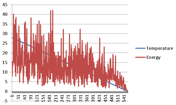
A sample tuning process can be depicted in the following figure where you can see that when the temperature is low, the solutions quickly converge.
–EOF (The Ultimate Computing & Technology Blog) —
1087 wordsLast Post: Include the Binary Files in Your Source Code
Next Post: Notes on Python again