In the field of machine learning and data mining, the Gradient Descent is one simple but effective prediction algorithm based on linear-relation data. It can be used to make prediction based on a large number of known data, for things like, predict heights given weights. This tutorial will guide you through the Gradient Descent via the C/C++ code samples.
Tutorial Data Set
For simplicity, we will use the following simple X/Y series for demonstration (so you can easily adapt to some real problems)
x y
1 1
2 3
4 3
3 2
5 5
Gradient Descent
There are many linear regression algorithms and Gradient Descent is one of the simplest method. For linear regression, you assume the data satisfies the linear releation, for example,
So, our task is to find the ‘optimal’ B0 and B1 such that the ‘prediction’ gives an acceptable accuracy. Let’s start the value of 0 for both B0 and B1.
So if we calculate the error for the first point  , we will have error = -1. Now can we use the error for Gradient Descent to update the weights. Since it is just 1 point, we can say that B0 is accountable for all the error. So we can tune B0 in this manner:

Where B0(t+1) is the updated version of the coefficient we will use on the next training instance (second point). The  is the learning rate and let’s pick a small number 0.01. So plug in these values, we will have:
 .
.
Now, for B1, it is slightly different, as we will need to take into account the value of x, so the formula becomes:

Let’s plug the values and we will have:

Now, we can iterately repeat the process to the next few instances until reaches the end, which is called 1 pass (an epoch). We can go round to the begining of the training instances as many times as we want to improve the accuracy of the model.
We can iterate this process 20 times that is 4 epoches. The process can be represented using the following C/C++ code.
double x[] = {1, 2, 4, 3, 5};
double y[] = {1, 3, 3, 2, 5};

double b0 = 0;
double b1 = 0;
double alpha = 0.01;

for (int i = 0; i < 20; i ++) {
    int idx = i % 5;
    double p = b0 + b1 * x[idx];
    double err = p - y[idx];
    b0 = b0 - alpha * err;
    b1 = b1 - alpha * err * x[idx];
}
So, if we print the values of b0, b1 and error, what do we get?
B0 = 0.01, B1 = 0.01, err = -1
B0 = 0.0397, B1 = 0.0694, err = -2.97
B0 = 0.066527, B1 = 0.176708, err = -2.6827
B0 = 0.0805605, B1 = 0.218808, err = -1.40335
B0 = 0.118814, B1 = 0.410078, err = -3.8254
B0 = 0.123526, B1 = 0.414789, err = -0.471107
B0 = 0.143994, B1 = 0.455727, err = -2.0469
B0 = 0.154325, B1 = 0.497051, err = -1.0331
B0 = 0.157871, B1 = 0.507687, err = -0.354521
B0 = 0.180908, B1 = 0.622872, err = -2.3037
B0 = 0.18287, B1 = 0.624834, err = -0.196221
B0 = 0.198544, B1 = 0.656183, err = -1.56746
B0 = 0.200312, B1 = 0.663252, err = -0.176723
B0 = 0.198411, B1 = 0.65755, err = 0.190068
B0 = 0.213549, B1 = 0.733242, err = -1.51384
B0 = 0.214081, B1 = 0.733774, err = -0.0532087
B0 = 0.227265, B1 = 0.760141, err = -1.31837
B0 = 0.224587, B1 = 0.749428, err = 0.267831
B0 = 0.219858, B1 = 0.735242, err = 0.472871
B0 = 0.230897, B1 = 0.790439, err = -1.10393
So, plotted visually:
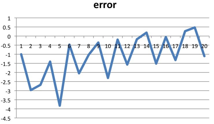
gradient-descent-error-prediction
From the graph, we can see that the error is gradually becoming smaller and our final model is:

If we make predictions using the given training instances (each point in our training dataset), we will have Root-Mean-Square-Error = 0.72.
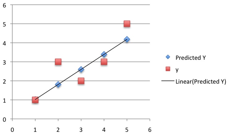
gradient-descent-prediction
Gradient descent method is normally used when having very large amounts of data, and it works quite well.
–EOF (The Ultimate Computing & Technology Blog) —
1084 wordsLast Post: The K Nearest Neighbor Algorithm (Prediction) Demonstration by MySQL
Next Post: How to Use Naive Bayes to Make Prediction (Demonstration via SQL) ?